Rolling GARCH Forecasts

The rugarch package contains a rolling volatility forecast function called ugarchroll, but in this example I will show how easy it is to create a quick custom function. Having a rolling forecast of volatility can prove an invaluable indicator for use in trading systems. an example of which is also included.

# The function makes exclusive use of xts based timeseries indexing.
garchv = function(x, start = 600, roll = 25, n.ahead = 1, spec = NULL, cluster = NULL)
{
# x : is a series of closing prices

# start : is the number of periods which are used for the first rolling
# estimation window

# roll : the number of periods to roll the 1-ahead forecast before
# re-estimating the model parameters

# n.ahead : the forecast horizon

# spec : the univariate GARCH model specification (uGARCHspec object)

# cluster : a pre-created cluster object from the parallel package
require(rugarch)
if (!is.xts(x))
stop('\nx must be an xts object')
# create continuous return series
r = na.omit(diff(log(x), 1))
n = nrow(r)
if (n <= start)
stop('\nstart cannot be greater than length of x')
# the ending points of the estimation window
s = seq(start + roll, n, by = roll)
m = length(s)
# the rolling forecast length
out.sample = rep(roll, m)
# adjustment to include all the datapoints from the end
if (s[m] < n) {
s = c(s, n)
m = length(s)
out.sample = c(out.sample, s[m] - s[m - 1])
}
# the default specification if none is provided is set to an eGARCH-std
# model
if (is.null(spec))
spec = ugarchspec(variance.model = list(model = 'eGARCH'), distribution = 'std')
if (!is.null(cluster)) {
clusterEvalQ(cluster, library(rugarch))
clusterEvalQ(cluster, library(xts))
clusterExport(cluster, varlist = c('r', 's', 'roll', 'spec', 'out.sample'),
envir = environment())
tmp = clusterApply(cl = cluster, 1:m, fun = function(i) {
fit = ugarchfit(spec, r[1:s[i], ], out.sample = out.sample[i], solver = 'hybrid')
f = ugarchforecast(fit, n.ahead = 1, n.roll = out.sample[i] - 1)
y = sigma(f)
# use xts for indexing the forecasts
y = xts(as.numeric(y), tail(time(r[1:s[i], ]), out.sample[i]))
return(y)
})
} else{
tmp = lapply(1:m, FUN = function(i) {
fit = ugarchfit(spec, r[1:s[i], ], out.sample = out.sample[i], solver = 'hybrid')
f = ugarchforecast(fit, n.ahead = 1, n.roll = out.sample[i] - 1)
y = sigma(f)
# use xts for indexing the forecasts
y = xts(as.numeric(y), tail(time(r[1:s[i], ]), out.sample[i]))
return(y)
})
}
# re-assemble the forecasts
forc = tmp[[1]]
for (i in 2:m) {
forc = rbind(forc, tmp[[i]])
}
colnames(forc) = 'V'
return(forc)
}

As an application of a rolling volatility forecast, I will consider the variable moving average (VMA) indicator of Chande (see Technical Analysis of Stocks & Commodities, March 1992), implemented in the TTR package.

getSymbols('SPY', src = 'yahoo', from = '1990-01-01')
SPY = adjustOHLC(SPY, use.Adjusted = TRUE)
library(parallel)
cluster = makePSOCKcluster(10)
garch_V = garchv(Cl(SPY), start = 600, roll = 25, n.ahead = 1, spec = NULL,
cluster = cluster)
stopCluster(cluster)

The VMA function uses a weighting vector, scaled between 0 and 1, with higher values (volatility) leading to faster adjustment of the moving average. Formally, it is defined as $$VM{A_t} = \left( {r{w_t}} \right){P_t} + \left( {1 – r{w_t}} \right)VM{A_{t – 1}}$$ where r is the decay ratio which adjusts the smoothness of the moving average, and w the weighting vector. In order to use the forecast volatility with the VMA indicator we need to rescale it to lie between the required bounds. A simple transformation which uses the min and max values can be used, such that $\bar h=\left(max(h)-h\right)/\left(\max(h)-min(h)\right)$. A slight problem with this approach is that the max and min of the forecast for the period is not known (not without looking ahead), but we ignore this problem at present.

barh = (garch_V - min(garch_V))/(max(garch_V) - min(garch_V))
tmp = cbind(Cl(SPY), barh)
tmp = na.omit(tmp)
VMA_garch1 = VMA(tmp[, 1], w = tmp[, 2]^2, ratio = 0.1)
VMA_garch2 = VMA(tmp[, 1], w = tmp[, 2]^2, ratio = 1)

For illustration, I’ll plot 2 VMA, a slow and fast version, the calibration of which is done through the decay ‘ratio’ option in the VMA function.

par(mfrow = c(2, 1))
plot(garch_V, main = 'SPY Volatility')
plot(tmp[, 1], main = 'SPY w/th VMA Indicator')
lines(VMA_garch1, col = 2)
lines(VMA_garch2, col = 4)

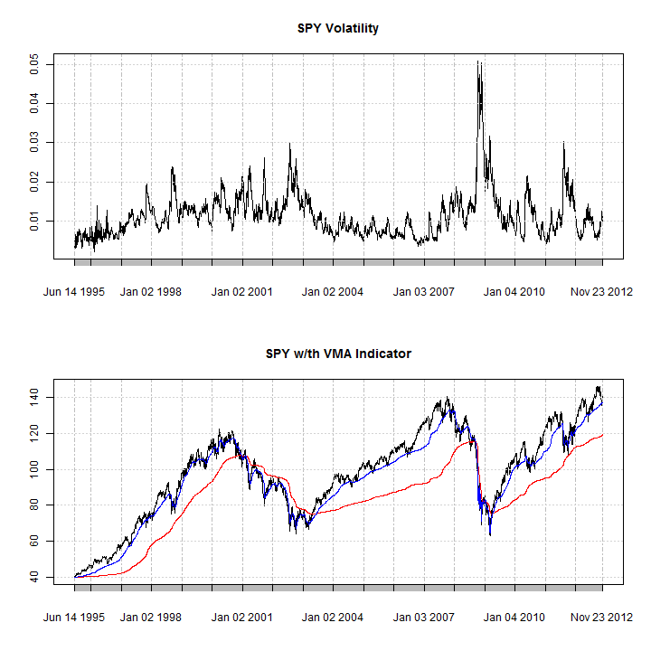
As can be visually inferred, the effect of the spikes in volatility on the moving average indicator are clearly illustrated, particularly around the 2008 period. A simple system would probably seek to be long the security when the fast moving average is above the slow moving average, when markets are trending.