In their paper on GARCH model comparison, Hansen and Lunde (2005) present evidence that among 330 different models, and using daily data on the DM/$ rate and IBM stock returns, no model does significantly better at predicting volatility (based on a realized measure) than the GARCH(1,1) model, for an out of sample period of about 250 days (between 1992/1993 for the currency, and 1999/2000 for the stock). In this demonstration, I instead ask if anything does NOT beat the GARCH(1,1) using a range of operational tests such as VaR exceedances, and model comparison using the model confidence set of Hansen, Lunde and Nason (2011) on a loss function based on the conditional quantiles. Using the S&P 500 index, and the latest 1500 days as the out of sample forecast period, I find that there are few models that do not beat the GARCH(1,1)-Normal.
Data Setup
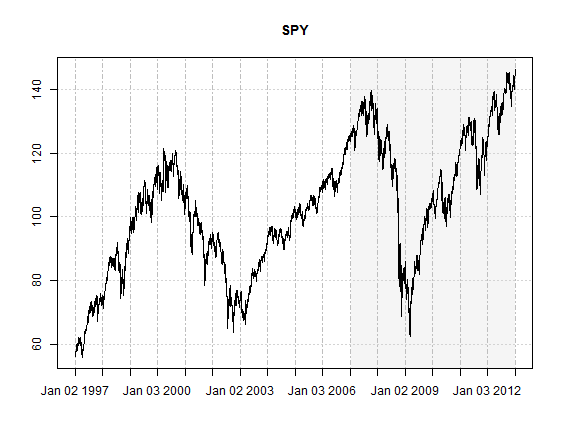
Given that it is the most widely cited and followed equity index in the world, the S&P 500 is a natural choice for testing a hypothesis, and for the purposes of this demonstration the log returns of the SPY index tracker were used. Starting on 23-01-2007, a rolling forecast and re-estimation scheme was adopted, with a moving window size of 1500 periods, and a re-estimation period of 50. The data was obtained from Yahoo finance and adjusted for dividends and splits.
library(rugarch)
library(shape)
library(xts)
library(quantmod)
getSymbols('SPY', from = '1997-01-01')
SPY = adjustOHLC(SPY, use.Adjusted = TRUE)
R = ROC(Cl(SPY), type = 'continuous', na.pad = FALSE)
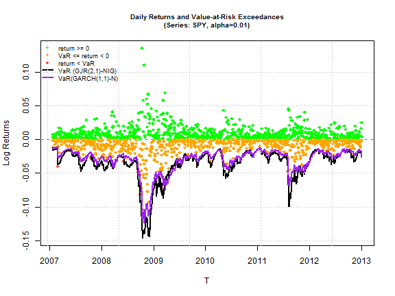
The following plot highlights the importance of the forecast period under consideration, which includes the credit crisis and an overall exceptional testing ground for risk model backtesting.
plot(Cl(SPY), col = 'black', screens = 1, blocks = list(start.time = paste(head(tail(index(SPY),1500), 1)), end.time = paste(index(tail(SPY, 1))), col = 'whitesmoke'), main = 'SPY', minor.ticks = FALSE)
Model Comparison
For the backtest the following GARCH models were chosen:
- GARCH
- GJR
- EGARCH
- APARCH
- component GARCH
- AVGARCH
- NGARCH
- NAGARCH
with four distributions, the Normal, Skew-Student (Fernandez and Steel version), Normal Inverse Gaussian (NIG) and Johnson’s SU (JSU). The conditional mean was based on an ARMA(2,1) model, while the GARCH order was set at (1,1) and (2,1), giving a total combination of 64 models. To create the rolling forecasts, the ugarchroll function was used, which has been completely re-written in the latest version of rugarch and now also includes a resume method for resuming from non-converged estimation windows.
model = c('sGARCH', 'gjrGARCH', 'eGARCH', 'apARCH', 'csGARCH', 'fGARCH', 'fGARCH', 'fGARCH')
submodel = c(NA, NA, NA, NA, NA, 'AVGARCH', 'NGARCH', 'NAGARCH')
spec1 = vector(mode = 'list', length = 16)
for (i in 1:8) spec1[[i]] = ugarchspec(mean.model = list(armaOrder = c(2, 1)), variance.model = list(model = model[i], submodel = if (i > 5) submodel[i] else NULL))
for (i in 9:16) spec1[[i]] = ugarchspec(mean.model = list(armaOrder = c(2, 1)), variance.model = list(garchOrder = c(2, 1), model = model[i - 8], submodel = if ((i - 8) > 5) submodel[i - 8] else NULL))
spec2 = vector(mode = 'list', length = 16)
for (i in 1:8) spec2[[i]] = ugarchspec(mean.model = list(armaOrder = c(2, 1)), variance.model = list(model = model[i], submodel = if (i > 5) submodel[i] else NULL), distribution = 'sstd')
for (i in 9:16) spec2[[i]] = ugarchspec(mean.model = list(armaOrder = c(2, 1)), variance.model = list(garchOrder = c(2, 1), model = model[i - 8], submodel = if ((i - 8) > 5) submodel[i - 8] else NULL), distribution = 'sstd')
spec3 = vector(mode = 'list', length = 16)
for (i in 1:8) spec3[[i]] = ugarchspec(mean.model = list(armaOrder = c(2, 1)), variance.model = list(model = model[i], submodel = if (i > 5) submodel[i] else NULL), distribution = 'nig')
for (i in 9:16) spec3[[i]] = ugarchspec(mean.model = list(armaOrder = c(2, 1)), variance.model = list(garchOrder = c(2, 1), model = model[i - 8], submodel = if ((i - 8) > 5) submodel[i - 8] else NULL), distribution = 'nig')
spec4 = vector(mode = 'list', length = 16)
for (i in 1:8) spec4[[i]] = ugarchspec(mean.model = list(armaOrder = c(2, 1)), variance.model = list(model = model[i], submodel = if (i > 5) submodel[i] else NULL), distribution = 'jsu')
for (i in 9:16) spec4[[i]] = ugarchspec(mean.model = list(armaOrder = c(2, 1)), variance.model = list(garchOrder = c(2, 1), model = model[i - 8], submodel = if ((i - 8) > 5) submodel[i - 8] else NULL), distribution = 'jsu')
spec = c(spec1, spec2, spec3, spec4)
cluster = makePSOCKcluster(15)
clusterExport(cluster, c('spec', 'R'))
clusterEvalQ(cluster, library(rugarch))
# Out of sample estimation
n = length(spec)
fitlist = vector(mode = 'list', length = n)
for (i in 1:n) {
tmp = ugarchroll(spec[[i]], R, n.ahead = 1, forecast.length = 1500, refit.every = 50, refit.window = 'moving', windows.size = 1500, solver = 'hybrid', calculate.VaR = FALSE, cluster = cluster, keep.coef = FALSE)
if (!is.null(tmp@model$noncidx)) {
tmp = resume(tmp, solver = 'solnp', fit.control = list(scale = 1), solver.control = list(tol = 1e-07, delta = 1e-06), cluster = cluster)
if (!is.null(tmp@model$noncidx))
fitlist[[i]] = NA
} else {
fitlist[[i]] = as.data.frame(tmp, which = 'density')
}
}
The method of using as.data.frame with option “density”, returns a data.frame with the forecast conditional mean, sigma, any skew or shape parameters for the estimation/forecast window, and the realized data for the period. Because I have made use of a time based data series, the returned data.frame has rownames the forecast dates.
| Date | Mu | Sigma | Skew | Shape | Shape (GIG) | Realized |
|---|---|---|---|---|---|---|
| 23/01/2007 | 0.00066 | 0.00496 | 0 | 0 | 0 | 0.00295 |
| 24/01/2007 | 0.00058 | 0.00487 | 0 | 0 | 0 | 0.008 |
| 25/01/2007 | 0.00025 | 0.00517 | 0 | 0 | 0 | -0.01182 |
| 26/01/2007 | 0.00074 | 0.00604 | 0 | 0 | 0 | -0.00088 |
| 29/01/2007 | 0.00087 | 0.00587 | 0 | 0 | 0 | -0.00056 |
| 30/01/2007 | 0.00086 | 0.00571 | 0 | 0 | 0 | 0.00518 |
| 31/01/2007 | 0.00063 | 0.00567 | 0 | 0 | 0 | 0.00666 |
| 01/02/2007 | 0.00033 | 0.00575 | 0 | 0 | 0 | 0.00599 |
| 02/02/2007 | 0.0001 | 0.0058 | 0 | 0 | 0 | 0.00141 |
| 05/02/2007 | 0.0001 | 0.00564 | 0 | 0 | 0 | 0.00024 |
In order to compare the models, the conditional coverage test for VaR exceedances of Christoffersen (1998) and the tail test of Berkowitz (2001) were used. The following code calculates the quantiles and applies the relevant tests described above.
vmodels = c('sGARCH(1,1)', 'gjrGARCH(1,1)', 'eGARCH(1,1)', 'apARCH(1,1)', 'csGARCH(1,1)','AVGARCH(1,1)', 'NGARCH(1,1)', 'NAGARCH(1,1)', 'sGARCH(2,1)', 'gjrGARCH(2,1)','eGARCH(2,1)', 'apARCH(2,1)', 'csGARCH(2,1)', 'AVGARCH(2,1)', 'NGARCH(2,1)','NAGARCH(2,1)')
modelnames = c(paste(vmodels, '-N', sep = ''), paste(vmodels, '-sstd', sep = ''), paste(vmodels, '-nig', sep = ''), paste(vmodels, '-jsu', sep = ''))
q1 = q5 = px = matrix(NA, ncol = 64, nrow = 1500)
dist = c(rep('norm', 16), rep('sstd', 16), rep('nig', 16), rep('jsu', 16))
# use apply since nig and gh distributions are not yet vectorized
for (i in 1:64) {
q1[, i] = as.numeric(apply(fitlist[[i]], 1, function(x) qdist(dist[i], 0.01, mu = x['Mu'], sigma = x['Sigma'], skew = x['Skew'], shape = x['Shape'])))
q5[, i] = as.numeric(apply(fitlist[[i]], 1, function(x) qdist(dist[i], 0.05, mu = x['Mu'], sigma = x['Sigma'], skew = x['Skew'], shape = x['Shape'])))
px[, i] = as.numeric(apply(fitlist[[i]], 1, function(x) pdist(dist[i], x['Realized'], mu = x['Mu'], sigma = x['Sigma'], skew = x['Skew'], shape = x['Shape'])))
}
VaR1cc = apply(q1, 2, function(x) VaRTest(0.01, actual = fitlist[[1]][, 'Realized'], VaR = x)$cc.LRp)
VaR5cc = apply(q5, 2, function(x) VaRTest(0.05, actual = fitlist[[1]][, 'Realized'], VaR = x)$cc.LRp)
BT1 = apply(px, 2, function(x) BerkowitzTest(qnorm(x), tail.test = TRUE, alpha = 0.01)$LRp)
BT5 = apply(px, 2, function(x) BerkowitzTest(qnorm(x), tail.test = TRUE, alpha = 0.05)$LRp)
VTable = cbind(VaR1cc, VaR5cc, BT1, BT5)
rownames(VTable) = modelnames
colnames(VTable) = c('VaR.CC(1%)', 'VaR.CC(5%)', 'BT(1%)', 'BT(5%)')
From a summary look at the head and tails of the tables, it is quite obvious that the GARCH(1,1)-Normal model is NOT hard to beat. More generally, the (1,1)-Normal models fare worst, and this is not surprising since financial markets, particularly for this crisis prone period under study, cannot possibly be well modelled without fat tailed and asymmetric distributions. A more interesting result is that the (2,1)-Non Normal models beat (1,1)-Non Normal models on average. Given the widely adopted (1,1) approach almost everywhere, this is a little surprising. It should however be noted that 1500 points where used for each estimation window…with less data, parameter uncertainty is likely to induce noise in a higher order GARCH model.
Top 10
| Model | VaR.CC(1%) | VaR.CC(5%) | BT(1%) | BT(5%) |
|---|---|---|---|---|
| AVGARCH(2,1)-sstd | 0.01 | 0.27 | 0.01 | 0.01 |
| AVGARCH(2,1)-nig | 0.17 | 0.18 | 0.12 | 0.03 |
| NAGARCH(2,1)-sstd | 0.11 | 0.18 | 0.1 | 0.02 |
| gjrGARCH(2,1)-sstd | 0.6 | 0.14 | 0.41 | 0.07 |
| NAGARCH(2,1)-nig | 0.25 | 0.14 | 0.13 | 0.04 |
| NAGARCH(2,1)-jsu | 0.36 | 0.14 | 0.23 | 0.05 |
| gjrGARCH(2,1)-nig | 0.6 | 0.14 | 0.45 | 0.13 |
| gjrGARCH(1,1)-jsu | 0.6 | 0.14 | 0.48 | 0.11 |
| gjrGARCH(2,1)-jsu | 0.6 | 0.14 | 0.55 | 0.12 |
| gjrGARCH(1,1)-nig | 0.6 | 0.14 | 0.39 | 0.13 |
Bottom 10
| Model | VaR.CC(1%) | VaR.CC(5%) | BT(1%) | BT(5%) |
|---|---|---|---|---|
| sGARCH(2,1)-N | 0 | 0 | 0 | 0 |
| NGARCH(2,1)-N | 0 | 0 | 0 | 0 |
| NGARCH(1,1)-N | 0 | 0 | 0 | 0 |
| csGARCH(1,1)-N | 0 | 0 | 0 | 0 |
| csGARCH(2,1)-N | 0 | 0 | 0 | 0 |
| apARCH(2,1)-N | 0 | 0 | 0 | 0 |
| sGARCH(1,1)-N | 0 | 0 | 0 | 0 |
| apARCH(1,1)-N | 0 | 0 | 0 | 0 |
| eGARCH(1,1)-N | 0 | 0 | 0 | 0 |
| eGARCH(2,1)-N | 0 | 0 | 0 | 0 |
The following plots provide for a clearer (hopefully!) visual representation of the results.
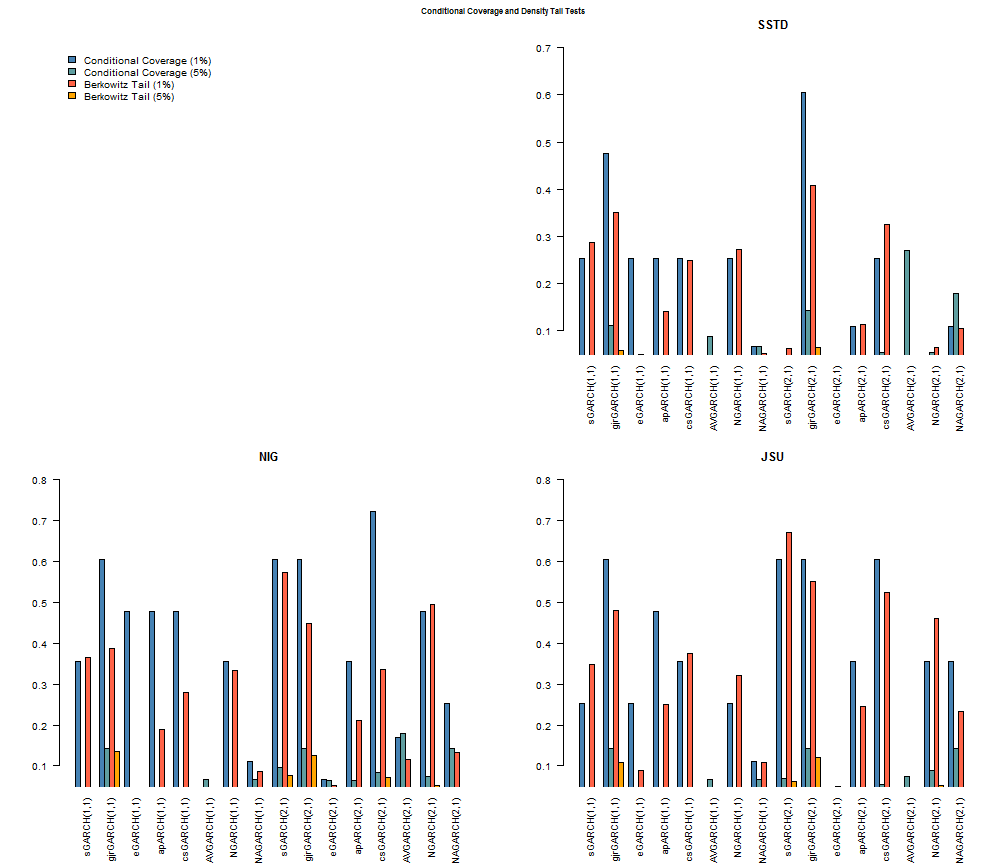
The models with conditional distribution the Normal are excluded since none of them are above the 5% significance cutoff. All other barplots start at 5% so that any bar which shows up indicates acceptance of the null of the hypothesis (for both tests this is phrased so that it indicates a correctly specified model). A careful examination of all the models indicates that the GJR (1,1) and (2,1) model from any of the 3 skewed and shaped conditional distributions passes all 4 tests. The SSTD distribution fares worst among the three, with the NIG and JSU appearing to provide an equally good fit. The final plot shows the VaR performance of the GARCH(1,1)-Normal and the GJR(2,1)-NIG for the period.
MCS Test on Loss Function
It is often said that the VaR exceedance tests are rather crude and require a lot of data in order to offer any significant insight into model differences. An alternative method for evaluating competing models is based on the comparison of some relevant loss function using a test such as the Model Confidence Set (MCS) of Hansen, Lunde and Nason (2011). In keeping with the focus on the tail of the distribution, a VaR loss function at the 1% and 5% coverage levels was used, described in González-Rivera et al.(2004) and defined as:
$${Q_{loss}} \equiv {N^{ – 1}}\sum\limits_{t = R}^T {\left( {\alpha – 1\left( {{r_{t + 1}} < VaR_{t + 1}^\alpha } \right)} \right)} \left( {{r_{t + 1}} – VaR_{t + 1}^\alpha } \right)$$
where \( P = T – R \) is the out-of-sample forecast horizon, \( T \) the total horizon to include in estimation, and \( R \) the start of the out-of-sample forecast. This is an asymmetric loss function, linearly penalizing exceedances more heavily by \( (1-\alpha) \). This is not yet exported in rugarch but can still be called as follows:
LossV5 = apply(q5, 2, function(x) rugarch:::.varloss(0.05, fitlist[[1]][, 'Realized'], x))
LossV1 = apply(q1, 2, function(x) rugarch:::.varloss(0.01, fitlist[[1]][, 'Realized'], x))
The MCS function is also not yet included, but may be in a future version. The following barplot shows the result of running the MCS test using a stationary bootstrap with 5000 replications.
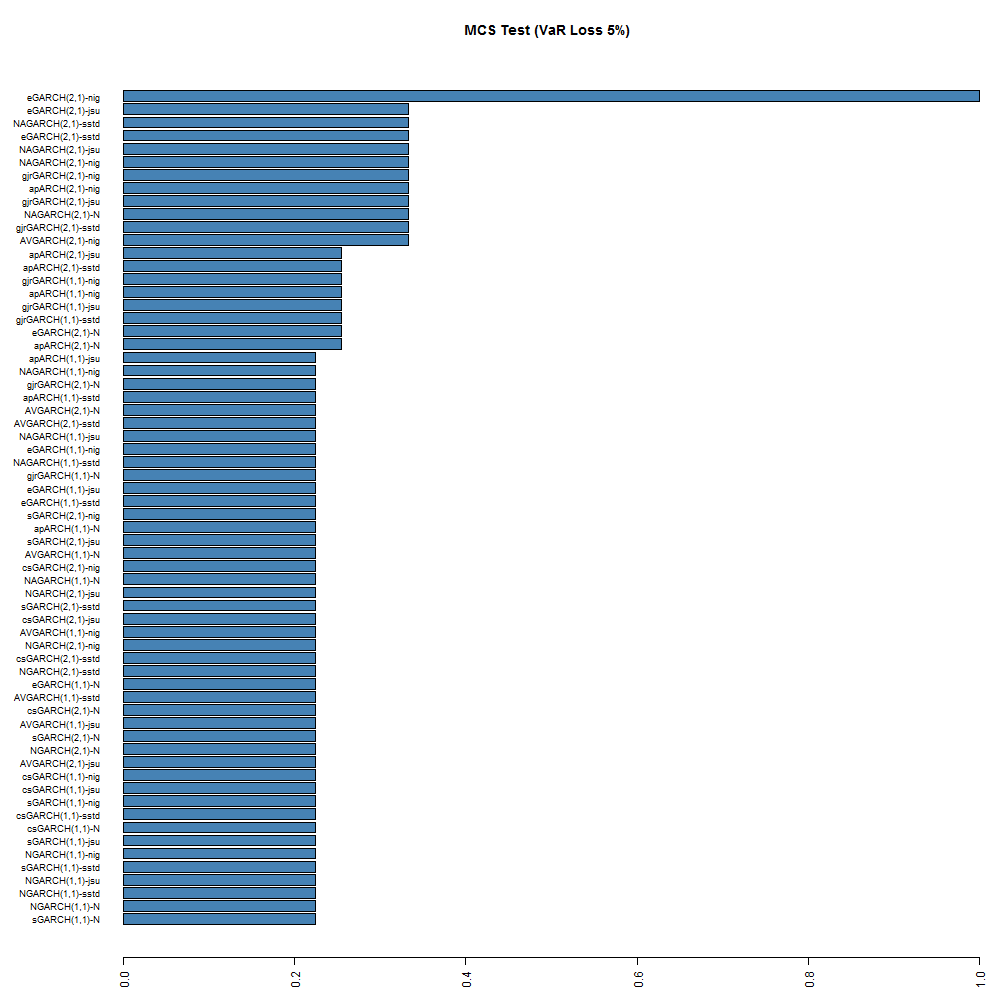
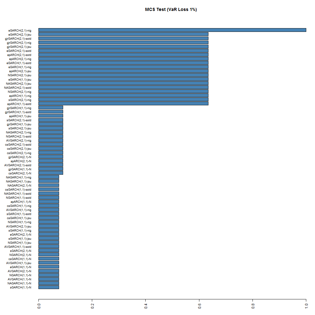
While no models are excluded from the model confidence set, at the 95% significance level, the ranking is still somewhat preserved for the top and bottom models, with the (2,1) NIG and JSU models being at the top. Based on this test, it would appear that the eGARCH(2,1)-NIG is the superior model at both coverage rates, with the GARCH(1,1)-Normal being at the very bottom with a 7% and 20% probability of belonging to the set at the 1% and 5% coverage rates respectively.
Conclusion
The normality assumption does not realistically capture the observed market dynamics, and neither does the GARCH(1,1)-N model. There were few models which did not beat it in this application. In fact, higher order GARCH models were shown to provide significant out performance on a range of tail related measures, and distributions such as the NIG and JSU appeared to provide the most realistic representation of the observed dynamics.
References
Berkowitz, J. (2001). Testing density forecasts, with applications to risk management. Journal of Business & Economic Statistics, 19(4), 465-474.
Christoffersen, P. F. (1998). Evaluating Interval Forecasts. International Economic Review, 39(4), 841-62.
González-Rivera, G., Lee, T. H., & Mishra, S. (2004). Forecasting volatility: A reality check based on option pricing, utility function, value-at-risk, and predictive likelihood. International Journal of Forecasting, 20(4), 629-645.
Hansen, P. R., & Lunde, A. (2005). A forecast comparison of volatility models: does anything beat a GARCH (1, 1)?. Journal of applied econometrics, 20(7), 873-889.
Hansen, P. R., Lunde, A., & Nason, J. M. (2011). The model confidence set. Econometrica, 79(2), 453-497.