VaR and Approximate VaR in the GO-GARCH (NIG) model.

This demonstration illustrates the calculation of the weighted (portfolio) VaR in the GO-GARCH (NIG/GH) model using both the semi-analytic convolution of weighted densities method as well as the Cornish-Fisher method using the weighted co-moments generated by the model. I am going to use the same setup as in the CAPM demonstration, so refer to that for more details.

library(rmgarch)
library(parallel)
library(xts)
data(dji30ret)
# investigate PCA
cl = makePSOCKcluster(10)
clusterEvalQ(cl, library(rmgarch))
X = as.xts(dji30ret)
spec = gogarchspec(mean.model = list(model = 'AR', lag = 1), variance.model = list(model = 'sGARCH',
    variance.targeting = TRUE), distribution = 'manig', ica = 'fastica')
mod2 = gogarchfit(spec, X, gfun = 'tanh', out.sample = 100, cluster = cl, maxiter1 = 1e+05,
    epsilon = 1e-07, rseed = 77, n.comp = 10)
forc2 = gogarchforecast(mod2, n.ahead = 1, n.roll = 99)

I’m not going to bother with in-sample estimation but will go directly to the forecast for this application (note that all methods are also applicable to goGARCHfit and goGARCHfilter objects). The following code shows how to generate the forecast quantile:

cf = convolution(forc2, weights = matrix(rep(1/30, 30), ncol = 30, nrow = 100),
    cluster = cl)
# create the weighted moments
fm = gportmoments(forc2, weights = matrix(rep(1/30, 30), ncol = 30, nrow = 100))
# Cornish Fisher Function
VaRCF = function(p = 0.01, mu, sigma, skew, kurt) {
    kurt = kurt - 3
    zc = qnorm(p)
    Zcf = zc + (1 - zc^2) * skew/6 + (zc^3 - 3 * zc) * kurt/24 + (5 * zc - 2 * zc^3) * (skew^2)/36
    VaR = mu + Zcf * sigma
    return(VaR)
}
VaR = matrix(NA, ncol = 4, nrow = 100)
colnames(VaR) = c('qfft[0.01]', 'cf[0.01]', 'qfft[0.05]', 'cf[0.05]')
for (i in 1:100) {
    # remember that this is zero base because of the roll indexed
    qfx = qfft(cf, index = i - 1)
    VaR[i, 1] = qfx(0.01)
    VaR[i, 2] = VaRCF(0.01, fm[1, 1, i], fm[1, 2, i], fm[1, 3, i], fm[1, 4,i])
    VaR[i, 3] = qfx(0.05)
    VaR[i, 4] = VaRCF(0.05, fm[1, 1, i], fm[1, 2, i], fm[1, 3, i], fm[1, 4,i])
}
VaR = xts(VaR, as.POSIXct(dimnames(fm)[[3]]))
par(mfrow = c(2, 1))
plot(VaR[, 1], main = 'VaR[1%] Forecast', cex.main = 0.9, auto.grid = FALSE, minor.ticks = FALSE, major.format = FALSE)
lines(VaR[, 2], col = 2)
legend('bottomleft', c('FFT based', 'Cornish-Fisher'), col = 1:2, lty = c(1,1), bty = 'n', cex = 0.8)
plot(VaR[, 3], main = 'VaR[5%] Forecast', cex.main = 0.9, auto.grid = FALSE, minor.ticks = FALSE, major.format = FALSE)
lines(VaR[, 4], col = 2)
legend('bottomleft', c('FFT based', 'Cornish-Fisher'), col = 1:2, lty = c(1,1), bty = 'n', cex = 0.8)

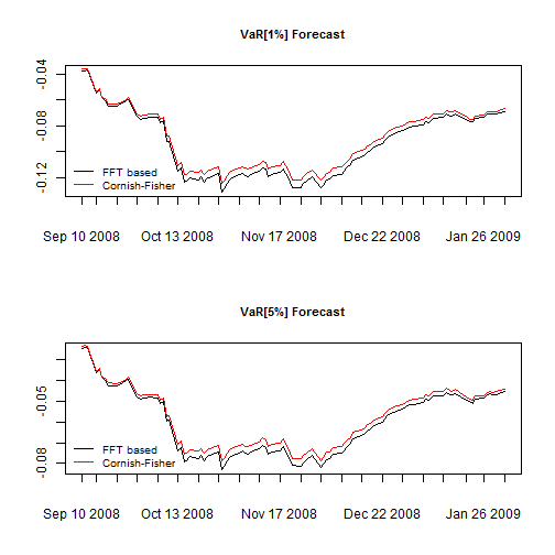
The two are quite close, and I suspect that with a larger number of assets, the two will be much closer as the weighted distribution approaches the normal.