This quick demonstration shows how to use specify a rugarch specification to estimate or filter a dataset using the exponentially weighted moving average model (EWMA). The EWMA model is a simple extension to the standard weighting scheme which assigns equal weight to every point in time for the calculation of the volatility, by assigning (usually) more weight to the most recent observations using an exponential scheme. This is effectively a restricted integrated GARCH (iGARCH) model, with the restriction that the intercept (\(\omega\)) is equal to zero, with the smoothing parameter (\(\lambda\)) equivalent to the autoregressive parameter (\(\beta\)) in the GARCH equation. \[
\sigma_t^2 =(1-\lambda)\varepsilon_{t-1}^2+\lambda\sigma_{t-1}^2
\] The \(\lambda\) parameter has sometimes been based on a specific rule of thumb value, advocated by Riskmetrics, depending on the frequency of the data (e.g. 0.94 for daily data), but we can just as easily estimate it. The demonstration shows how to pass a fixed value for lambda or estimate it, and a comparison with an unrestricted model for the S&P 500 series. Note that we estimate \(\alpha\) in the iGARCH model and set \(\beta=1-\alpha\).
require(rugarch)
require(xts)
data(sp500ret)
ewma.spec.fixed = ugarchspec(mean.model=list(armaOrder=c(0,0), include.mean=FALSE),
variance.model=list(model="iGARCH"), fixed.pars=list(alpha1=1-0.94, omega=0))
ewma.spec.est = ugarchspec(mean.model=list(armaOrder=c(0,0), include.mean=FALSE),
variance.model=list(model="iGARCH"), fixed.pars=list(omega=0))
igarch.spec = ugarchspec(mean.model=list(armaOrder=c(0,0), include.mean=FALSE),
variance.model=list(model="iGARCH"))
mod1 = ugarchfit(ewma.spec.fixed, as.xts(sp500ret))
mod2 = ugarchfit(ewma.spec.est, as.xts(sp500ret))
mod3 = ugarchfit(igarch.spec, as.xts(sp500ret))
plot(sigma(mod3), main="", auto.grid = FALSE, major.ticks = "auto",
minor.ticks = FALSE)
lines(sigma(mod2), col=2, lty=2)
lines(sigma(mod1), col=3, lty=3)
cf1=round(coef(mod2)[3],3)
l1 = as.expression("iGARCH")
l2 = as.expression(substitute(paste("EWMA[est.",lambda,"=",x,"]"), list(x=cf1)))
l3 = as.expression(substitute(paste("EWMA[fix.",lambda,"=",x,"]"), list(x=0.94)))
legend("topright", c(l1, l2, l3), col=1:3, lty=1:3, bty="n", cex=0.9)
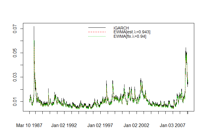
EWMA Comparison Plot
Not too surprising, the 3 plots look very similar and the estimated \(\lambda\) parameter is identical to the rule of thumb value of 0.94. Notice that the first model which has all parameters fixed was not estimated but instead dispatched to the ugarchfilter method with a warning.