At the recent R/Finance 2014 conference in Chicago I gave a talk on Smooth Transition AR models and a new package for estimating them called twinkle. In this blog post I will provide a short outline of the models and an introduction to the package and its features.
Financial markets have a strong cyclical component linked to the business cycle, and may undergo temporary or permanent shifts related to both endogenous and exogenous shocks. As a result, the distribution of returns is likely to be different depending on which state of the world we are in. It is therefore advantageous to model such dynamics within a framework which can accommodate and explain these different states. Within time series econometrics, the switching between states has been based either on unobserved components, giving rise to the Markov Switching (MS) models introduced by Hamilton (1989), or observed components leading to Threshold type Autoregressive (TAR) models popularized by Tong (1980). This post and the accompanying package it introduces considers only observed component switching, though there are a number of good packages in R for Markov Switching.
The Smooth Transition AR Model
The smooth transition AR model was introduced in Teräsvirta (1994), and has been used in numerous studies from GDP modelling to forex and equity market volatility. See the presentation from the talk above which includes a number of selected references.
The s-state model considered in the twinkle package takes the following form:
\[
{y_t} = \sum\limits_{i = 1}^s {\left[ {\left( {{{\phi ‘}_i}y_t^{\left( p \right)} + {{\xi ‘}_i}{x_t} + {{\psi ‘}_i}e_t^{\left( q \right)}} \right){F_i}\left( {{z_{t – d}};{\gamma _i},{\alpha _i},{c_i},{\beta _i}} \right)} \right]} + {\varepsilon _t}
\]
where:
\[
\begin{gathered}
y_t^{\left( p \right)} = {\left( {1,\tilde y_t^{\left( p \right)}} \right)^\prime },\quad \tilde y_t^{\left( p \right)} = {\left( {{y_{t – 1}}, \ldots ,\quad {y_{t – p}}} \right)^\prime },{\phi _i} = {\left( {{\phi _{i0}},{\phi _{i1}}, \ldots ,\quad {\phi _{ip}}} \right)^\prime } \\
\varepsilon _t^{\left( q \right)} = {\left( {{\varepsilon _{t – 1}}, \ldots ,\quad {\varepsilon _{t – q}}} \right)^\prime },{{\psi ‘}_i} = {\left( {{\psi _{i1}}, \ldots ,{\psi _{iq}}} \right)^\prime }\\
{x_t}{\text{ }} = {\left( {{x_1}, \ldots ,{x_l}} \right)^\prime },\quad {{\xi ‘}_i}{\text{ }} = {\left( {{\xi _{i1}}, \ldots ,{\xi _{il}}} \right)^\prime } \\
\end{gathered}
\]
and we allow for a variance mixture so that \( {\varepsilon _t} \sim iid\left( {0,{\sigma _i},\eta } \right) \) with \( \eta \) denoting any remaining distributional parameters which are common across states. The softmax function is used to model multiple states such that:
\[
\begin{gathered}
{F_i}\left( {{z_{t – d}};{\gamma _i},{\alpha _i},{c_i},{\beta _i}} \right) = \frac{{{e^{{\pi _{i,t}}}}}}
{{1 + \sum\limits_{i = 1}^{s – 1} {{e^{{\pi _{i,t}}}}} }} \\
{F_s}\left( {{z_{t – d}};{\gamma _i},{\alpha _i},{c_i},{\beta _i}} \right) = \frac{1}
{{1 + \sum\limits_{i = 1}^{s – 1} {{e^{{\pi _{i,t}}}}} }}\\
\end{gathered}
\]
where the state dynamics \( \pi_{i,t} \) also include the option of lag-1 autoregression:
\[
{\pi _{i,t}} = {\gamma _i}\left( {{{\alpha ‘}_i}{z_{t – d}} – {c_i}} \right) + {{\beta ‘}_i}{\pi _{i,t – 1}},\quad \gamma_i>0
\]
with initialization conditions given by:
\[\pi _{i,0} = \frac{{{\gamma _i}\left( {{{\alpha ‘}_i}\bar z – {c_i}} \right)}}{{1 – {\beta _i}}},\quad \left| \beta \right| < 1\]
The parameter \( \gamma_i \) is a scaling variable determining the smoothness of the transition between states, while \( c_i \) is the threshold intercept about which switching occurs.
The transition variable(s) \( z_t \) may be a vector of external regressors each with its own lag, or a combination of lags of \( y_t \) in which case the model is ‘rudely’, as one participant in the conference noted, called ‘self-exciting’. Should \( z_t \) be a vector, then for identification purposes \( \alpha_1 \) is fixed to 1. Additionally, as will be seen later, it is also possible to pass a function \( f\left(.\right) \) which applies a custom transformation to the lagged values in the case of the self-exciting model. While it may appear at first that the same can be achieved by pre-transforming those values and passing the transformed variables in the switching equation, this leaves you dead in the water when it comes to s(w)imulation and n-ahead forecasting where the value of the transition variable depends on the lagged simulated value of that same variable.
Finally, the transition function \( F_i \) has usually been taken to be either the logistic or exponential transform functions. As the 2 figures below illustrate, the logistic nests the TAR model as \( \gamma_i\to \infty \) and collapses to the linear case as \( \gamma_i\to 0 \). The exponential on the other hand collapses to the linear case as \( \gamma_i \) approaches the limits and has a symmetric shape which is sometimes preferred for exchange rate modelling because of the perceived symmetric exchange rate adjustment behavior. Currently, only the logistic is considered in the twinkle package.
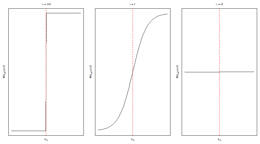
Logistic Transition
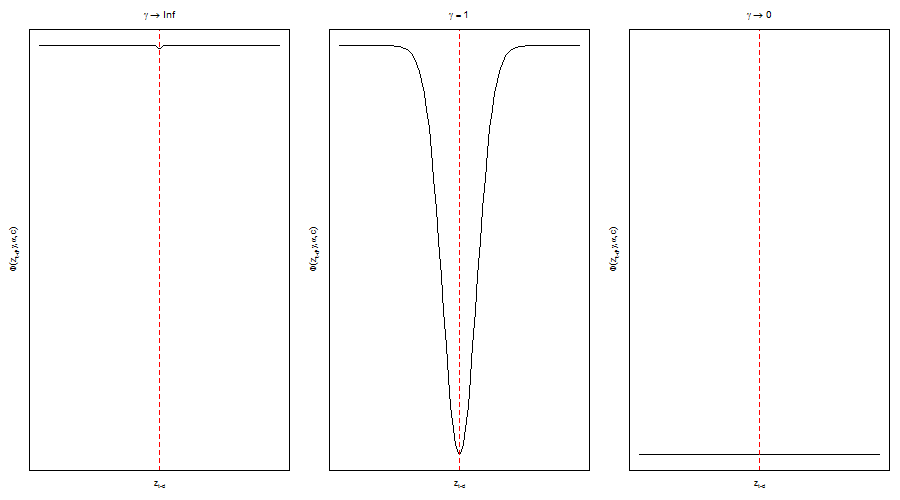
Exponential Transition
Implementation
I follow a similar construction paradigm for the twinkle package as I have in my other packages. Namely, an S4 framework which includes steps for specifying the model, estimation, inference and tests, visual diagnostics, filtering, forecasting, simulation and rolling estimation/forecasting. I consider these to be the minimum methods for creating a complete modelling environment for econometric analysis. Additional methods are summarized in the following table:
| Method | Description | Class | Example |
|---|---|---|---|
| setfixed<- | Set fixed parameters | [1] | >setfixed(spec)<-list(s1.phi0=0) |
| setstart<- | Set starting parameters | [1] | >setstart(spec)<-list(s1.phi0=0) |
| setbounds<- | Set parameter bounds | [1] | >setbounds(spec)<-list(s1.phi0=c(0,1)) |
| nonlinearTest | Luukkonen Test | [1][2] | >nonlinearTest(fit, robust=TRUE) |
| modelmatrix | model matrix | [1][2] | >modelmatrix(fit, linear=FALSE) |
| coef | coef vector | [2][3] | >coef(fit) |
| fitted | conditional mean | [2][3][4][5][6] | >fitted(fit) |
| residuals | residuals | >residuals(fit) | |
| states | conditional state probabilities | [2][3][4][5][6] | >states(fit) |
| likelihood | log likelihood | [2][3] | >likelihood(fit) |
| infocriteria | normalized information criteria | [2][3][7] | >infocriteria(fit) |
| vcov | parameter covariance matrix | [2] | >vcov(fit) |
| convergence | solver convergence | [2][7] | >convergence(fit) |
| score | numerical score matrix | [2] | >score(fit) |
| sigma | conditional sigma | [2][3][4][5][6] | >sigma(fit) |
| as.data.frame | conditional density | [7] | >as.data.frame(roll) |
| quantile | conditional quantiles | [2][3][4][5][6][7] | >quantile(fit) |
| pit | conditional probability integral transformation | [2][3][7] | >pit(fit) |
| show | summary | [1][2][3][4][5][6][7] | >fit |
The classes in column 3 are: [1] STARspec, [2] STARfit, [3] STARfilter, [4] STARforecast, [5] STARsim, [6] STARpath, [7] rollSTAR.
Model Specification
The model specification function has a number of options which I will briefly discuss in the section.
args(starspec)
#
## function (mean.model = list(states = 2, include.intercept = c(1,
##     1), arOrder = c(1, 1), maOrder = c(0, 0), matype = 'linear',
##     statevar = c('y', 's'), s = NULL, ylags = 1, statear = FALSE,
##     yfun = NULL, xreg = NULL, transform = 'logis'), variance.model = list(dynamic = FALSE,
##     model = 'sGARCH', garchOrder = c(1, 1), submodel = NULL,
##     vreg = NULL, variance.targeting = FALSE), distribution.model = 'norm',
##     start.pars = list(), fixed.pars = list(), fixed.prob = NULL,
##     ...)
##
Mean Equation
Upto 4 states may be modelled, with a choice of inclusion or exclusion of an intercept in each state (include.intercept), the number of AR (arOrder) and MA (maOrder) parameters per state and whether to include external regressors in each state (xreg should be a prelagged xts matrix). Note that the default for the moving average terms is to include them outside the states, but this can be changed by setting matype=’state’. The statevar denotes what the state variable is, with “y” being the self-exciting model and “s” a set of external regressors passed as a prelagged xts matrix to s. If the choice is “y”, the ylags should be a vector of the lags for the variable with a choice like c(1,3) denoting lag-1 and lag-3. Finally, the yfun option was discussed in the previous section and is a custom transformation function for y returning the same number of points as given.
Variance Equation
The variance can be either static (default) or dynamic (logical), in which case it can be one of 3 GARCH models (‘sGARCH’,’gjrGARCH’ or ‘eGARCH’) or ‘mixture’ as discussed previously. The rest of the options follow from those in the rugarch package in the case of GARCH type variance.
Other options
The same distributions as those in rugarch are implemented, and there is the option of passing fixed or starting parameters to the specification, although the methods ‘setfixed< –‘ and ‘setstart<-‘ allow this to be set once the specification has been formed. There is also a ‘setbounds<-‘ method for setting parameter bounds which for the unconstrained solvers (the default to use with this type of model) means using a logistic bounding transformation. Finally, the fixed.probs option allows the user to pass a set of fixed state probabilities as an xts matrix in which case the model is effectively linear and may be estimated quite easily.
Parameter naming
It is probably useful to have the naming convention of the parameters used in the package should starting, fixed or bounds need to be set. These are summarized in the list below and generally follow the notation used in the representation of the model in the previous section:
- All state based variables are preceded by their state number (s1.,s2.,s3.,s4.)
- Conditional Mean Equation:
- intercept: phi0 (e.g. s1.phi0, s2.phi0)
- AR(p): phi1, …, phip (e.g. s1.phi1, s1.phi2, s2.phi1, s2.phi2)
- MA(q): psi1, …, psiq (e.g. s1.psi1, s1.psi2, s2.psi1, s2.psi2). Note that in the case of matype=’linear’, the states are not used.
- X(l): xi1, …, xil (e.g. s1.xi1, s2.xi2, x3.xi1)
- State Equation:
- scaling variable: gamma (e.g. s1.gamma)
- Threshold: c (e.g. s1.c)
- Threshold Variables (k): alpha2, …, alphak (e.g. s1.alpha2, s1.alpha3). Note that the first variable (alpha1) is constrained to be 1 for identification purposes so cannot be changed. This will always show up in the summary with NAs in the standard errors since it is not estimated.
- Threshold AR(1): beta (e.g. s1.beta)
- Variance Equation:
- sigma (s): If dynamic and mixture then s1.sigma, s2.sigma etc. If static then just sigma.
- GARCH parameters follow same naming as in the rugarch package
- Distribution:
- skew
- shape
I’ll define a simple specification to use with this post and based on examples from the twinkle.tests folder in the src distribution (under the inst folder). This is based on a weekly realized measure of the Nasdaq 100 index for the period 02-01-1996 to 12-10-2001, and the specification is for a simple lag-1 self-exciting model with AR(2) for each state.
require(quantmod)
data(ndx)
ndx.ret2 = ROC(Cl(ndx), na.pad = FALSE)^2
ndx.rvol = sqrt(apply.weekly(ndx.ret2, FUN = 'sum'))
colnames(ndx.rvol) = 'RVOL'
spec = starspec(mean.model = list(states = 2, arOrder = c(2, 2), statevar = 'y',
ylags = 1))
Before proceeding, I also check the presence of STAR nonlinearity using the test of Luukkonen (1988) which is implemented in the nonlinearTest method with an option for also testing with the robust assumption (to heteroscedasticity):
tmp1 = nonlinearTest(spec, data = log(ndx.rvol))
tmp2 = nonlinearTest(spec, data = log(ndx.rvol), robust = TRUE)
testm = matrix(NA, ncol = 4, nrow = 2, dimnames = list(c('Standard', 'Robust'),
c('F.stat', 'p.value', 'Chisq.stat', 'p.value')))
testm[1, ] = c(tmp1$F.statistic, tmp1$F.pvalue, tmp1$chisq.statistic, tmp1$chisq.pvalue)
testm[2, ] = c(tmp2$F.statistic, tmp2$F.pvalue, tmp2$chisq.statistic, tmp2$chisq.pvalue)
print(testm, digit = 5)
##
##          F.stat   p.value Chisq.stat   p.value
## Standard 3.7089 0.0014366     21.312 0.0016123
## Robust   2.5694 0.0193087     15.094 0.0195396
We can safely reject the linearity assumption under the standard test at the 1% significance level, and under the robust assumption at the 5% significance level. Note that this example is taken from the excellent book of Zivot (2007) (chapter on nonlinear models) and the numbers should also agree with what is printed there.
Model Estimation
Estimating STAR models is a challenging task, and for this purpose a number of options have been included in the package.
args(starfit)
#
## function (spec, data, out.sample = 0, solver = 'optim', solver.control = list(),
##     fit.control = list(stationarity = 0, fixed.se = 0, rec.init = 'all'),
##     cluster = NULL, n = 25, ...)
## NULL
The data must be an xts object with the same time indices as any data already passed to the STARspec object and contain only numeric data without any missing values. The out.sample is used to indicate how many data points to optionally leave out in the estimation (from the end of the dataset) for use in out-of-sample forecasting later on when the estimated object is passed to the starforecast routine. Perhaps the most important choice to be made is the type of solver to use and it’s control parameters solver.control which should not be omitted. The following solvers and ‘strategies’ are included:
- optim. The preferred choice is the BFGS solver. The choice of solver is controlled by the method option in the solver.control list. All parameter bounds are enforced through the use of a logistic transformation.
- nlminb. Have had little luck getting the same performance as the BFGS solver.
- solnp. Will most likely find a local solution.
- cmaes. Even though it is a global solver, it requires careful tweaking of the control parameters (and there are many). This is the parma package version of the solver.
- deoptim. Another global solver. May be slow and require tweaking of the control parameters.
- msoptim. A multistart version of optim with option for using the cluster option for parallel evaluation. The number of multi-starts is controlled by the n.restarts option in the solver.control list.
- strategy. A special purpose optimization strategy for STAR problems using the BFGS solver. It cycles between keeping the state variables fixed and estimating the linear variables (conditional mean, variance and any distribution parameters), keeping the linear variables fixed and estimating the state variables, and a random re-start optimization to control for possibly local solutions. The argument n in the routine controls the number of times to cycle through this strategy. The solver.control list should pass control arguments for the BFGS solver. This is somewhat related to concentrating the sum of squares methodology in terms of the estimation strategy, but does not minimize the sum of squares, opting instead for a proper likelihood evaluation.
The strategy and msoptim solver strategies should be the preferred choice when estimating STARMA models.
I continue with the example already covered in the specification section and estimate the model, leaving 50 points for out of sample forecasting and filtering later on:
mod = starfit(spec, data = log(ndx.rvol), out.sample = 50, solver = 'strategy',
n = 8, solver.control = list(alpha = 1, beta = 0.4, gamma = 1.4, reltol = 1e-12))
show(mod)
plot(mod)
#
##
## *---------------------------------*
## *          STAR Model Fit         *
## *---------------------------------*
## states       : 2
## statevar     : y
## statear      : FALSE
## variance     : static
## distribution : norm
##
##
## Optimal Parameters (Robust Standard Errors)
## ------------------------------------
##            Estimate  Std. Error    t value Pr(>|t|)
## s1.phi0    -3.54380    0.034260 -103.43760 0.000000
## s1.phi1    -0.64567    0.426487   -1.51393 0.130043
## s1.phi2     0.10950    0.319605    0.34262 0.731886
## s2.phi0    -2.51982    0.849927   -2.96475 0.003029
## s2.phi1     0.10902    0.214009    0.50944 0.610444
## s2.phi2     0.17944    0.062210    2.88447 0.003921
## s1.gamma    3.22588    1.941072    1.66190 0.096532
## s1.c       -2.52662    0.347722   -7.26620 0.000000
## s1.alpha1   1.00000          NA         NA       NA
## sigma       0.39942    0.019924   20.04776 0.000000
##
## LogLikelihood : -126.3
##
## Akaike       1.0738
## Bayes        1.1999
## Shibata      1.0714
## Hannan-Quinn 1.1246
##
## r.squared         :  0.3167
## r.squared (adj)   :  0.2913
## RSS               :  40.2
## skewness (res)    :  -0.235
## ex.kurtosis (res) :  0.4704
##
## AR roots
##         Moduli1 Moduli2
## state_1   1.274   7.170
## state_2   2.076   2.684
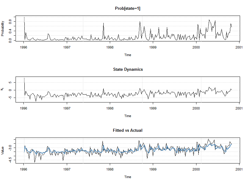
plot(mod)
Model Filtering
Filtering a dataset with an already estimated set of parameters has been already extensively discussed in a related post for the rugarch package. The method takes the following arguments:
args(starfilter)
##
## function (spec, data, out.sample = 0, n.old = NULL, rec.init = 'all', ...)
##
The most important argument is probably n.old and denotes, in the case that the new dataset is composed of the old dataset (on which estimation took place) and the new data, the number of points composing the original dataset. This is so as to use the same initialization values for certain recursions and return the exact same results for those points in the original dataset. The following example illustrates:
specf = spec
setfixed(specf) < - as.list(coef(mod))
N = nrow(ndx.rvol) - 50
modf = starfilter(specf, data = log(ndx.rvol), n.old = N)
print(all.equal(fitted(modf)[1:N], fitted(mod)))
## [1] TRUE
print(all.equal(states(modf)[1:N], states(mod)))
## [1] TRUE
Model Forecasting
Nonlinear models are considerable more complex than their linear counterparts to forecast. For 1-ahead this is quite simple, but for n-ahead there is no closed form solution as in the linear case. Consider a general nonlinear first order autoregressive model:
\[
{y_t} = F\left( {{y_{t – 1}};\theta } \right) + {\varepsilon _t}
\]
The 1-step ahead forecast is simply:
\[
{{\hat y}_{t + 1\left| t \right.}} = E\left[ {{y_{t + 1}}\left| {{\Im _t}} \right.} \right] = F\left( {{y_t};\theta } \right)
\]
However, for n-step ahead, and using the Chapman-Kolmogorov relationship \( g\left( {{y_{t + h}}\left| {{\Im _t}} \right.} \right) = \int_{ – \infty }^\infty {g\left( {{y_{t + h}}\left| {{y_{t + h – 1}}} \right.} \right)g\left( {{y_{t + h – 1}}\left| {{\Im _t}} \right.} \right)d{y_{t + h – 1}}} \), we have:
\[E\left[ {{y_{t + h}}\left| {{\Im _t}} \right.} \right] = \int_{ – \infty }^\infty {E\left[ {{y_{t + h}}\left| {{y_{t + h – 1}}} \right.} \right]g\left( {{y_{t + h – 1}}\left| {{\Im _t}} \right.} \right)d{y_{t + h – 1}}}\]
where there is no closed form relationship since \( E\left[ {F\left( . \right)} \right] \ne F\left({E\left[ . \right]} \right) \).
The trick is to start at h=2:
\[
{{\hat y}_{t + 2\left| t \right.}} = \frac{1}{T}\sum\limits_{i = 1}^T {F\left( {{{\hat y}_{t + 1\left| t \right.}} + {\varepsilon _i};\theta } \right)}
\]
and using either quadrature integration or monte carlo summation obtain the expected value. Use that value for the next step, rinse and repeat.
In the twinkle package, both quadrature and monte carlo summation are options in the starforecast method:
args(starforecast)
#
## function (fitORspec, data = NULL, n.ahead = 1, n.roll = 0, out.sample = 0,
##     external.forecasts = list(xregfor = NULL, vregfor = NULL,
##         sfor = NULL, probfor = NULL), method = c('an.parametric',
##         'an.kernel', 'mc.empirical', 'mc.parametric', 'mc.kernel'),
##     mc.sims = NULL, ...)
## NULL
with added options for either parametric, empirical or kernel fitted distribution for the residuals. The method also allows for multiple dispatch methods by taking either an object of class STARfit or one of class STARspec (with fixed parameters and a dataset). The example below illustrates the different methods:
forc1 = starforecast(mod, n.roll = 2, n.ahead = 20, method = 'an.parametric',
mc.sims = 10000)
forc2 = starforecast(mod, n.roll = 2, n.ahead = 20, method = 'an.kernel', mc.sims = 10000)
forc3 = starforecast(mod, n.roll = 2, n.ahead = 20, method = 'mc.empirical',
mc.sims = 10000)
forc4 = starforecast(mod, n.roll = 2, n.ahead = 20, method = 'mc.parametric',
mc.sims = 10000)
forc5 = starforecast(mod, n.roll = 2, n.ahead = 20, method = 'mc.kernel', mc.sims = 10000)
show(forc1)
par(mfrow = c(2, 3))
plot(forc1)
plot(forc2)
plot(forc3)
plot(forc4)
plot(forc5)
#
##
## *------------------------------------*
## *        STAR Model Forecast         *
## *------------------------------------*
## Horizon        : 20
## Roll Steps     : 2
## STAR forecast  : an.parametric
## Out of Sample  : 20
##
## 0-roll forecast [T0=2000-10-27]:
##      Series
## T+1  -2.684
## T+2  -2.820
## T+3  -2.948
## T+4  -3.061
## T+5  -3.157
## T+6  -3.231
## T+7  -3.286
## T+8  -3.324
## T+9  -3.350
## T+10 -3.368
## T+11 -3.379
## T+12 -3.387
## T+13 -3.392
## T+14 -3.395
## T+15 -3.397
## T+16 -3.398
## T+17 -3.399
## T+18 -3.400
## T+19 -3.400
## T+20 -3.400
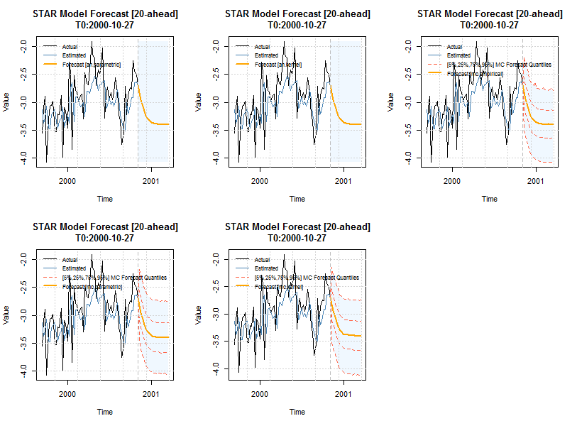
The nice thing about the monte carlo method is that the density of each point forecast is now available, and used in the plot method to draw quantiles around that forecast. It can be extracted by looking at the slot object@forecast$yDist, which is list of length n.roll+1 of matrices of dimensions mc.sims by n.ahead.
Model Simulation
Simulation in the twinkle package, like in rugarch, can be carried out directly on the estimated STARfit object else on a specification object of class STARspec with fixed parameters. Achieving equivalence between the two relates to start-up initialization conditions and is always a good check on reproducibility and code correctness, and shown in the example that follows:
sim = starsim(mod, n.sim = 1000, rseed = 10)
path = starpath(specf, n.sim = 1000, prereturns = tail(log(ndx.rvol)[1:N], rseed = 10)
all.equal(fitted(sim), fitted(path))
## TRUE
all.equal(states(sim), states(path))
## TRUE
The fitted method extracts the simulated series as an n.sim by m.sim matrix, while the states method extracts the simulated state probabilities (optionally takes “type” argument with options for extracting the simulated raw dynamics or conditional simulated mean per state) and can be passed the argument sim to indicate which m.sim run to extract (default: 1). Passing the correct prereturns value and the same seed as in starsim, initializes the simulation from the same values as the test of equality shows between the 2 methods. Things become a little more complicated when using external regressors or GARCH dynamics, but with careful preparation the results should again be the same.
Rolling estimation and 1-step ahead forecasting
The final key modelling method, useful for backtesting, is that of the rolling estimation and 1-step ahead forecasting which has a number of options to define the type of estimation window to use as well as a resume method which re-estimates any windows which did not converge during the original run. This type of method has already been covered in related posts of rugarch so I will reserve a more in-depth demo for a later date.
Final Thoughts
This post provided an introduction to the use of the twinkle package which should hopefully make it to CRAN from bitbucket soon. It is still in beta, and it will certainly take some time to mature, so please report bugs or feel free to contribute patches. The package departs from traditional implementations, sparse as they are, in the area of STAR models by offering extensions in the form of (MA)(X) dynamics in the conditional mean, (AR) dynamics in the conditional state equation, a mixture model for the variance, and a softmax representation for the multi-state model. It brings a complete modelling framework, developed in the rugarch package, to STAR model estimation with a set of methods which are usually lacking elsewhere. It also brings, at least for the time being, a promise of user engagement (via the R-SIG-FINANCE mailing list) and maintenance.
Download
Download and installation instructions can be found here.
References
[1] Hamilton, J. D. (1989). A new approach to the economic analysis of nonstationary time series and the business cycle. Econometrica: Journal of the Econometric Society, 357-384.
[2] Tong, H., & Lim, K. S. (1980). Threshold Autoregression, Limit Cycles and Cyclical Data. Journal of the Royal Statistical Society. Series B (Methodological), 245-292.
[3] Teräsvirta, T. (1994). Specification, estimation, and evaluation of smooth transition autoregressive models. Journal of the American Statistical association, 89(425), 208-218.
[4] Luukkonen, R., Saikkonen, P., & Teräsvirta, T. (1988). Testing linearity against smooth transition autoregressive models. Biometrika, 75(3), 491-499.
[5] Zivot, E., & Wang, J. (2007). Modeling Financial Time Series with S-PLUS® (Vol. 191). Springer.